
NOTE: At the time of writing, this package was available within Dalhousie Physical Oceanography only on our IBM RISC System/6000 machines.
Although Data Explorer is an easy package to learn to use, tutorials have been created that let you quickly learn some of the basics. Although this tutorial was designed for users at Dalhousie Physical Oceanography, it was be useful to other DX users as well.
Videos on Creating Visual Programs and Data Importing and Module Writing are available. The IBM Visualization Data Explorer manuals (User's Guide, User's Reference, and Programmer's Reference) are also available.
Data Explorer has a extensive on-line help facility, which is basically a copy of the User's Reference. This can be accesses by pressing the middle mouse button on a module or any window.
Other sources of information on the Internet include:
Tutorial 1: Viewing Topology/Bathemetry Data
We will build this visualization using modules, a pre-defined set of programs that manipulate data. When connected together, these modules form a program, or network diagram, that we will run to create an image.
NOTE: At the time of writing, Data Explorer is only available (within Dalhousie Physical Oceanography) on our IBM RISC System/6000 machines.
The Visual Program Editor window should appear on the screen. It will look like this:
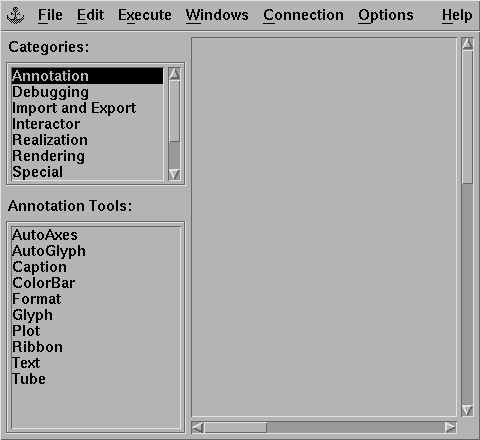
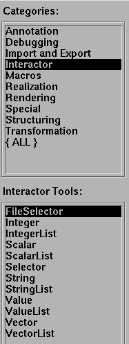
To use the FileSelector module, go to the left of the Visual Program Editor window, and under Categories, select Interactor. Then below it, under Interactor Tools:, select FileSelector (as seen in the diagram below).
Move the mouse pointer to the right into the main work area. Position the mouse where you want to put the FileSelector module (usually at the top when beginning a program, you can change it later if necessary by clicking and holding the left mouse button on the module, and then moving it to the desired location), then click the left mouse button once. A small green box should appear (see diagram below), with the word "FileSelector" in it. This is called a module.

NOTE: There are two outputs from the FileSelector module. The left tab will output the filename with the complete pathname, and the right tab outputs only the filename. The left one will be used in this example, and is generally the most useful output.
To select a filename using the FileSelector module, double click the left mouse button on the module and a new window should appear (see diagram below).
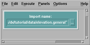
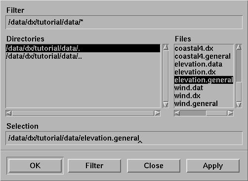
Type in the filename "/data/dx/tutorial/data/elevation.general", or you can click on the "..." button, which will bring up another new window (see diagram below). In this new window you can select a file by clicking on the file list on the right. You can also change the pathname by clicking on the list on the left.
NOTE:
The Name parameter is usually connected to the output tab of a File Selector module, to make selecting the file easier and less prone to typing errors. Alternatively you can specify the name of the file you wish to import here.
The format parameter is the type of file to import. This defaults to (file extension or content), which means that it will automatically change depending on the filename selected. It should be always be left as the default. Possible values for this field are "dx" (Data Explorer's own file format), "cdf" (NetCDF file format), and "general" (a general file format used with the Data Explorer "dx -prompter" command, see manual for further information on this).
Tabs that are already set (i.e. the tab is pointing in towards the module, or the parameter is greyed out) can be unset simply by double clicking on the module to get the parameters of that module. Then click on the little box on the left beside the parameter name on unset the parameter.
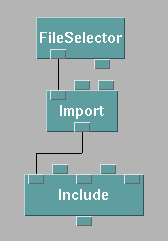
Connect the left output tab of the FileSelector module to the Name parameter of the Import module. To accomplish this, click and hold the left mouse button on the bottom left tab of the FileSelector module. The name of the tab that you you are on will appear in the module box (it should read "FileSelector filename"). While still holding the left mouse button, drag the mouse to the leftmost input tab of Import. The name of the tab that you are going to connect to appears in the module box (it should read "name Import"). Now release the mouse, and a line should now be connecting the two modules.
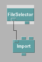
The above diagram has the output tab of FileSelector connected to the name input of Import. Note the tabs that are set are inside of the module, and the tabs that are not set are outside of the module.
NOTE: Most of the other options of Import are automatically changed depending on the filename selected, and changing them from their defaults may cause an error. We will use the defaults in this tutorial.
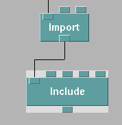
Connect the output tab of Import with the data input of the Include module.
The max parameter sets the upper limit of data to be used. Any data value higher that this will be excluded.
The exclude parameter is a flag that will reverse the way the module works and will exclude data values between min and max. This parameter is not set by default.
The cull parameter is a flag that if set to 0 will mark the points as invalid, and if set to 1 will remove the points. It is set to 1 by default. This will sometimes cause problems because it will make the grid irregular, so setting this flag to 0 is a good idea.
Now set the parameters of the Include module. We will set min to -400, and set cull to 0, causing all points below -400 to be marked invalid. By not setting a max value, it will default to the maximum data value in the file.
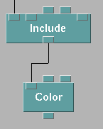
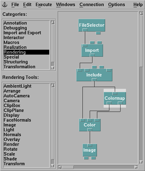
Join the output tab of the Include module with the input tab of the Color module.
The Color parameter is the color to change the data. This can be input from the rgb output tab of the ColorMap module, or can be entered directly. Valid colors can be entered as a vector (i.e. [r g b], where r is red, g is green, and b is blue, between 0 and 1, like [0.5 0.5 0.5] which is a shade of grey, or [1 1 0] which is yellow). Colors can also be entered as "red", "black", "limegreen", etc.
The opacity parameter sets the translucency of the object. This parameter can also be input from the opacity output tab of the ColorMap module, or can be a value from 0 to 1. A value of 0 means that the object is completely transparent, and a value of 1 means that the object is opaque.
We will not alter the input parameters of color until the ColorMap module.
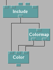
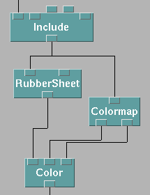
Now connect the output tab of Include to the input of ColorMap. Include is already connected to the output tab of the Color module, but each module's output tab may be connected to several other modules.
Now connect the rgb output tab of ColorMap to the Color input of Color. Then connect the opacity output of ColorMap to the opacity input of Color. This will allow the ColorMap module to control the coloring of the data.
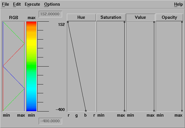
NOTE: The minimum and maximum values will only be automatically set after the program is executed and an image is formed. You might have to alter the colors after this first part of the tutorial has been completed to see these effects.
The default is to color the data values from red to blue, with red assigned to the highest data value and blue to the lowest.
To change the colors, you can move the anchor points (the little boxes on the line) in the Hue window. To create new anchor points, double click anywhere in the Hue window, and a new anchor will appear, along with the data value at that point on the side. The same can be done with the Saturation and Value windows. These add white and black respectively to the color. Experiment with these to get the desired color. The same can be done for the Opacity window.
The colormap for this tutorial might appear as follows:
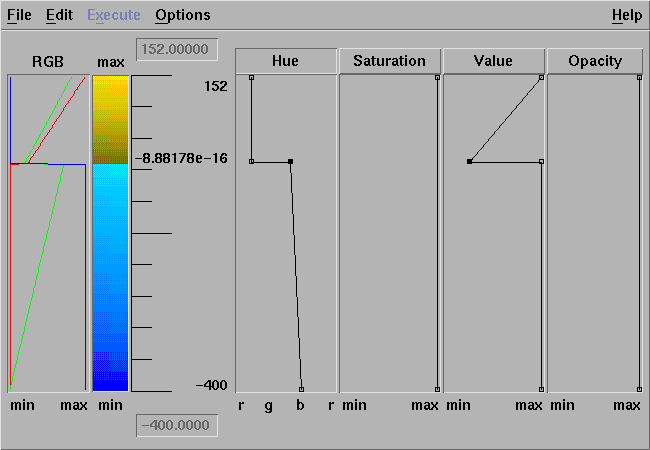
Image has only one parameter, the object input. Connect the output tab of Color to this tab. The output tabs of this module are hardly ever used.
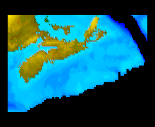
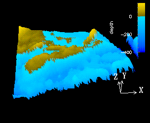
The resulting image from the tutorial should appear as follows. Your results may vary depending on the colors you chose in the ColorMap Editor.

In this tutorial we will augment the program from the first tutorial by making the image appear 3D and by adding vectors to the image. We will also add a color bar to the image, which will help to decipher what the colors on the image represent.
The position parameter tells us where in the Image Window to place the color bar. It is a vector with an x and y component, with values between 0 and 1. A value of [0 0] would put the color bar in the lower left corner, and [1 1] would put it in the upper right corner.
The shape parameter is the size that the color bar will appear in the Image Window. This is also a 2-vector, representing an x and y component in pixels.
The horizontal parameter is a flag that controls the direction of the color bar. The default of 0 would mean to make the color bar go down, and a value of 1 would mean to make it go across.
The label parameter just the title of the color bar. You can set this appropriately.
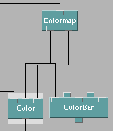
Double click on the ColorBar module, and set the following parameters:
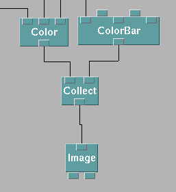
Collect's only parameter are objects. If you wish to add more objects, click on the Collect module, then go the Edit menu at the top and select Add Input Tab. This will create another input tab on the Collect module, allowing you to add another object to collect with the other inputs. This can be done to a maximum of 21 objects.
Join the output tab of ColorBar to the one of the input tabs of Collect, then do the same with Color and the other input tab of Collect. Disconnect the line joining Color and Image by clicking on the input tab of Image, dragging the line into empty space, and then releasing the mouse button. Now join the output tab of Collect to the input tab of Image.
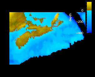
Now Execute the program, and the new image should contain a color bar in the upper right corner of the image, as shown below:
The scale parameter adjusts the scale factor of the deformation. If the image appears to deformed, lower the scale parameter. If the image appears to be a flat surface, increase the scale parameter.
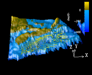
Set the scale parameter to 0.30. Now Execute the program. You should not notice any difference. This is because you are looking at the image from above. To change the view from which you are looking at the image, go to the Options menu of the Image Window (make sure you do this from the Image Window, as the Option menu there are different from the Options menu in the Visual Program Editor window). Select View Control and the View Control window will appear:
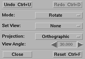
Change the Mode to Rotate and go to the Image Window. You will now notice a co-ordinate plane with the X, Y, and Z axis labelled (Z comes out of the screen). You can click the left mouse button and move the mouse to change the orientation of the image. This will allow you to see the 3D look of the image, as shown here:
NOTE: Other Modes that might be useful are Zoom and Pan/Zoom. Using the left mouse button and selecting an outline will zoom in on that area, while using the right mouse button and doing the same thing will zoom out. The difference between Zoom and Pan/Zoom is that Zoom will always zoom in on the center of the Image window, and Pan/Zoom will let you choose the point on which to center the zoom.
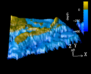
The method parameter alters the way the module adds normals. This defaults to "positions", which is what one would normally use.
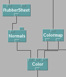
Execute and note the change in the image, as shown here:
New data must be imported for the surface current vectors. Select and then connect the following modules:
The which parameter is the number of the member you want to choose. We will choose the default 0, to choose the first frame of the multi-frame series.
The type parameter defines what kind of arrow to display. This is useful for making 2D vectors into 3D looking arrows, by specifying "rocket". Other useful values are "arrow" and "needle".Normally this is left as the default which will determine the appropriate type of arrow to display.
The shape parameter sets the thickness of the arrow. Set this to 1.4 for this example.
The scale parameter sets increase or decreases the length of the arrow.
The ratio parameter is the ratio between the lengths of the largest and the smallest arrows. If this value is set to 1, all arrows will be the same length. This value is normally kept at 0, and should be set at 0 for this example.
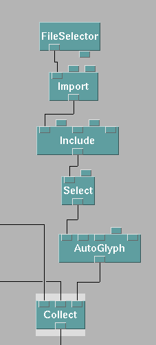
Execute and a set of vectors showing surface current should be displayed on the image.

Now go to the Select module and change the which parameter to 1 and Execute. This will change the data to the second frame of data. This is not practical for viewing many frames of data, so we will use another module called Sequencer.

and then clicking on the "..." button.
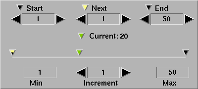
Other buttons on the Sequencer window work like VCR buttons. Refer to the manual for a more in depth discussion of how these buttons work.
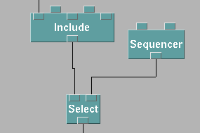
Set the max of Sequencer to 49 and the min to 0. Next, bring up the Sequencer window as described above, then hit the "play" button (arrow pointing right). The vectors on the image should now change direction and magnitude. You can use the other buttons to play backward, pause, or stop.
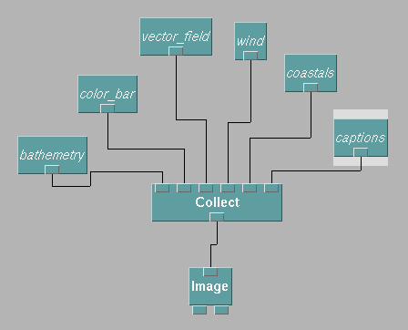
To start, we will disconnect the lines connecting Color (the one attached to Normals) and Collect. Place a Transmitter module under Color, and a Receiver above Collect. These will have default names, but changing them will be much more descriptive and helpful in the future. Double-click on Transmitter and change the Notation field at the top to bathemetry. Any receivers that had the old name will automatically change to the new name. Now connect the Color module to the Transmitter module.
Do the same the outputs listed below and any necessary receivers:
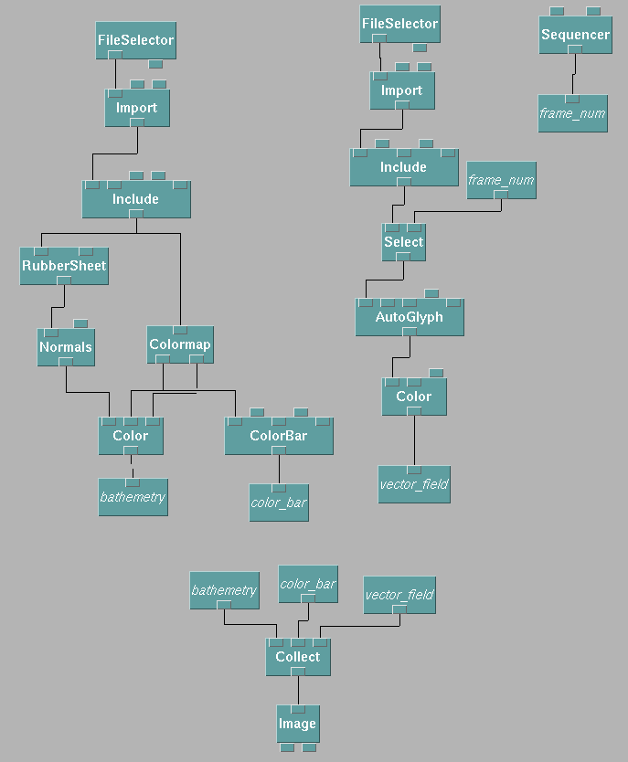
In this tutorial we will add some different vectors and we will also add text to the screen that tells us the time of frame being displayed.
To add a wind vector, we do much the same as the vector field. Select and connect the following modules, and enter the options listed.
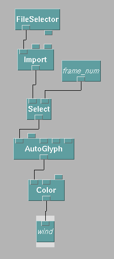
NOTE: only one Sequencer is allowed per program, therefore the same Sequencer must be used for parts of the program.
Choose and connect a Receiver to the Collect module. Change its notation parameter to wind (the same as the transmitter).
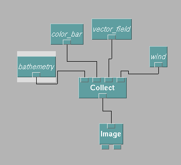
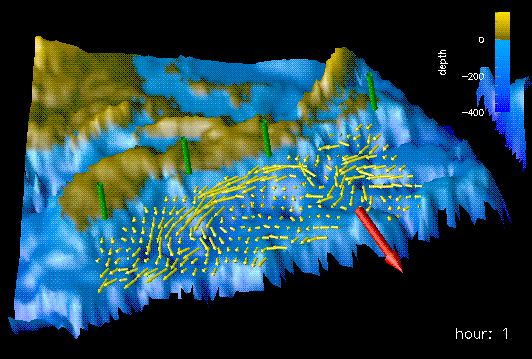
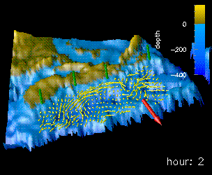
Execute the program again and now you should see a big red wind vector where Sable Island is located.
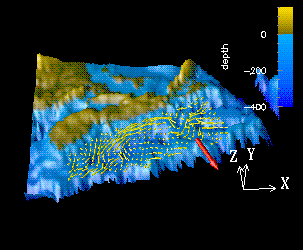
Do the same thing 3 more times using the filenames: coastal2.general, coastal3.general, and coastal4.general. Each of these files contains 50 frames of sea surface height data, each at a distinct shoreline location. Join the four sub-programs using a Collect module.
Now choose a Receiver and attach it to the which parameter of the Select module of each sub-program. Double-click on the Receiver module and change the notation to frame_num.
It should look like this:
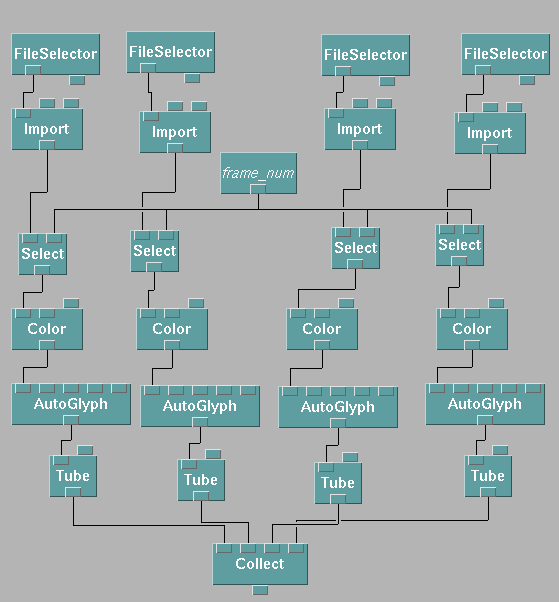
Since all of the sub-programs each do the same thing with the data, we can delete three of the Color modules, three of the AutoGlyph modules, and three of the Tube modules. Connect the remaining modules to look like this:
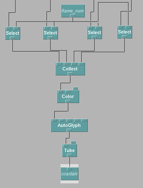
Select a Transmitter module, name it coastals, and connect the output of Tube to its input (as shown above).
Select a Receiver module, name it coastals, and attach it to the Collect module that is attached to Image.
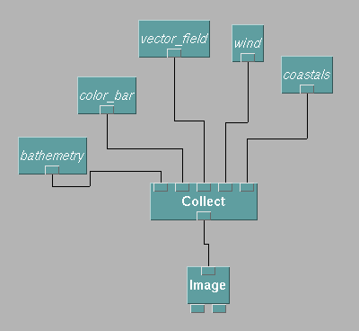
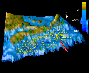
Execute the program again and you should now see the four green sea surface height indicators.
The value parameter is the value to insert into a %d, %f, or %s. This parameter is optional.
The position parameter works the same as the position parameter for the ColorBar module.
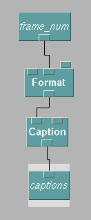
Select a Receiver module, and name it captions, and attach it to the Collect module that is attached to Image.
Execute the program to see the final results of this data visualization program:
