|
|
Bokeh Quickstart |
Bokeh 5-minute Overview
Bokeh is a Python interactive visualization library that targets modern web browsers for presentation. Its goal is to provide elegant, concise construction of novel graphics in the style of D3.js, and to extend this capability with high-performance interactivity over very large or streaming datasets. Bokeh can help anyone who would like to quickly and easily create interactive plots, dashboards, and data applications.
Simple Example
Here is a simple first example. First we'll import the figure function from bokeh.plotting, which will let us create all sorts of interesting plots easily. We also import the show and ouptut_notebook functions from bokeh.io — these let us display our results inline in the notebook.
from bokeh.plotting import figure
from bokeh.io import output_notebook, show
Next, we'll tell Bokeh to display its plots directly into the notebook. This will cause all of the Javascript and data to be embedded directly into the HTML of the notebook itself. (Bokeh can output straight to HTML files, or use a server, which we'll look at later.)
output_notebook()
Next, we'll import NumPy and create some simple data.
from numpy import cos, linspace
x = linspace(-6, 6, 100)
y = cos(x)
Now we'll call Bokeh's figure function to create a plot p. Then we call the circle() method of the plot to render a red circle at each of the points in x and y.
We can immediately interact with the plot:
- click-drag will pan the plot around.
- mousewheel will zoom in and out (after enabling in the toolbar)
The toolbar below is the default one that is available for all plots. It can be configured further via the tools keyword argument.
p = figure(width=500, height=500)
p.circle(x, y, size=7, color="firebrick", alpha=0.5)
show(p)
Bar Plot Example
Bokeh's core display model relies on composing graphical primitives which are bound to data series. This is similar in spirit to D3, and different than most other Python plotting libraries.
A slightly more sophisticated example demonstrates this idea.
Bokeh ships with a small set of interesting "sample data" in the bokeh.sampledata package. We'll load up some historical automobile mileage data, which is returned as a Pandas DataFrame.
from bokeh.sampledata.autompg import autompg

grouped = autompg.groupby("yr")

mpg = grouped.mpg
avg, std = mpg.mean(), mpg.std()
years = list(grouped.groups)
american = autompg[autompg["origin"]==1]
japanese = autompg[autompg["origin"]==3]
For each year, we want to plot the distribution of MPG within that year.
p = figure(title="MPG by Year (Japan and US)")

p.vbar(x=years, bottom=avg-std, top=avg+std, width=0.8,
       fill_alpha=0.2, line_color=None, legend_label="MPG 1 stddev")

p.circle(x=japanese["yr"], y=japanese["mpg"], size=10, alpha=0.5,
         color="red", legend_label="Japanese")

p.triangle(x=american["yr"], y=american["mpg"], size=10, alpha=0.3,
           color="blue", legend_label="American")

p.legend.location = "top_left"
show(p)
This kind of approach can be used to generate other kinds of interesting plots. See many more examples in the Bokeh Documentation Gallery.
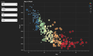
Linked Brushing
To link plots together at a data level, we can explicitly wrap the data in a ColumnDataSource. This allows us to reference columns by name.
We can use a "select" tool to select points on one plot, and the linked points on the other plots will highlight.
from bokeh.models import ColumnDataSource
from bokeh.layouts import gridplot

source = ColumnDataSource(autompg)

options = dict(width=300, height=300,
               tools="pan,wheel_zoom,box_zoom,box_select,lasso_select")

p1 = figure(title="MPG by Year", **options)
p1.circle("yr", "mpg", color="blue", source=source)

p2 = figure(title="HP vs. Displacement", **options)
p2.circle("hp", "displ", color="green", source=source)

p3 = figure(title="MPG vs. Displacement", **options)
p3.circle("mpg", "displ", size="cyl", line_color="red", fill_color=None, source=source)

p = gridplot([[ p1, p2, p3]], toolbar_location="right")

show(p)
You can read more about the ColumnDataSource and other Bokeh data structures in Providing Data for Plots and Tables
Standalone HTML
In addition to working well with the Notebook, Bokeh can also save plots out into their own HTML files. Here is the bar plot example from above, but saving into its own standalone file.
Now when we call show(), a new browser tab is also opened with the plot. If we just wanted to save the file, we would use save() instead.
from bokeh.plotting import output_file

output_file("barplot.html")

p = figure(title="MPG by Year (Japan and US)")

p.vbar(x=years, bottom=avg-std, top=avg+std, width=0.8,
       fill_alpha=0.2, line_color=None, legend_label="MPG 1 stddev")

p.circle(x=japanese["yr"], y=japanese["mpg"], size=10, alpha=0.3,
         color="red", legend_label="Japanese")

p.triangle(x=american["yr"], y=american["mpg"], size=10, alpha=0.3,
           color="blue", legend_label="American")

p.legend.location = "top_left"
show(p)
Bokeh Applications
Bokeh also has a server component that can be used to build interactive web applications that easily connect the powerful constellation of PyData tools to sophisticated Bokeh visualizations. The Bokeh server can be used to:
- respond to UI and tool events generated in a browser with computations or queries using the full power of python
- automatically push server-side updates to the UI (i.e. widgets or plots in a browser)
- use periodic, timeout, and asynchronous callbacks to drive streaming updates
The cell below shows a simple deployed Bokeh application from https://demo.bokeh.org embedded in an IFrame. Scrub the sliders or change the title to see the plot update.
from IPython.display import IFrame
IFrame('https://demo.bokeh.org/sliders', width=900, height=410)
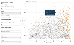
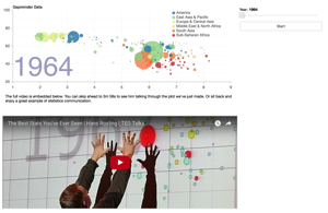
Click on any of the thumbnails below to launch other live Bokeh applications.
Find more details and information about developing and deploying Bokeh server applications in the User's Guide chapter Running a Bokeh Server.
