1: Introduction
2: Invoking Gre
3: Gre Grammar
4: Commands
5: Cookbook
6: Hints
7: History
8: Plans
9: Concept Index

1: Introduction

1.1: What ``gre`' is

`Gre' is a program for making science graphs. It is a programming language, not a GUI-based application. `Gre' is analagous to textual markup languages, such as TeX, LaTeX, HTML, etc. This analogy points out the pros and cons of `gre'. Pro: users get good control over the output graphs. Con: users must climb a learning curve before using `gre'.

`Gre' is based on the `Gri' `Gri' language. The main differences between the two are that `gre' is faster that `gre' has a simpler, more powerful, syntax. `Gre' syntax is based on the Perl language (Perl programmers).

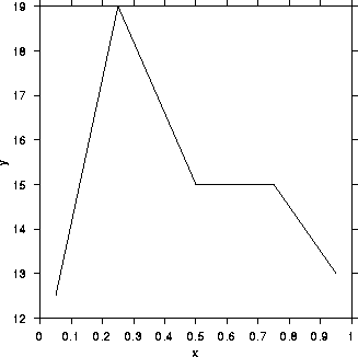
1.2: A simple example

To try `gre', do the following.

Create a datafile by inserting the following text into a file called `example1.dat':
```
   0.05 12.5
   0.25 19
   0.5  15
   0.75 15
   0.95 13
```
This is a datafile. Each line has an `(x,y)' pair. If you don't know what an `(x,y)' pair is, `gre' may not be what you need for your work!
Create a command-file by inserting the following text into in a file called `example1.gre':
```
   open example1.dat;
   read columns x=1 y=2;
   draw curve;
```
This is a `gre' program with three commands. Commands are separated by semicolons; in this case they are also separated by line separators, but these are optional, as is all whitespace in a `gre' program. The commands do the following things.
1. The first command opens the indicated data-file.
2. The second command reads `x' data from the first column and `y' data from the second column.
3. The third command indicates to draw the ``curve'' formed by the `(x,y)' points provided in the data-file. The curve comprises connected line segments -- it is not smoothed, although the word ``curve'' might fool you that it is!
Before the curve is drawn, axes will also be drawn (see below).
Run `gre' by typing
```
   gre example1
```
to the operating system. `Gre' assumes the commandfile has suffix `.gre', so there is no need to supply the suffix, although nothing is lost if you do supply it.

The three-line program makes use of many default `gre' actions, e.g. automatic drawing of axes and automatic selection of scales. All defaults may be overridden. The following example illustrates how to get `gre' to call the y-axis `foo' instead of `y', and to make this axis range from `0' to `20', labelled at intervals of `10', instead of `12' to `19' labelled at unit intervals (the x-axis still being selected automatically by `gre'):

   open example1.dat;
   read columns x=1 y=2;
   set y name "foo";
   set y axis 0 20 10;
   draw curve;

For more on `set y axis', see Set y axis.

A note on execution order. Notice that these axis-control commands were placed before the `draw curve' command. This illustrates an important point: `gre' executes the commands in a command-file sequentially, starting at the top. If, for example, the commands for controlling the y-axis were placed after the `draw curve' command, they would have no effect on this graph.

Note for Matlab users: The `gre' convention of executing commands in sequence agrees with most programming languages except Matlab. In matlab, some commands work non-sequentially, e.g. an `axis' command can change an existing graph. However, other Matlab commands (basically, all non-drawing commands) act sequentially ... imagine how confusing it would be if arithmetic commands acted out of sequence, as some Matlab graphics commands do!

1: Introduction

1.1: What `gre' is

1.2: A simple example

1.1: What ``gre`' is