The current version of CANDIE uses the Arakawa A grid formulation. It
was developed by Dan Wright. The main reason for choosing the A grid
CANDIE as our standard model code is based on the finding that the
C-grid model does not reproduce well the bottom trapped baroclinic
topographic Rossby waves in a periodic channel with a uniformly
slopping bottom. The governing equations and time discretization used
on the A grid CANDIE are identical to the C grid (see Sections A.1 and
A.2). The main differences between the A-grid and C-grid formations
are solely associated with the spatial discretization of horizontal
velocity components u and v. On the A grid u and v are
defined at the center of each cell (i.e., the p points, see Figure
1). On the C grid, on the other hand, u and v are defined on the
cell faces normal to the x and y directions, respectively.
The A grid formulation overcomes the difficulty of the C-grid in
estimating the Coriolis terms since the state variables u and v
are defined at the same location. The conservation equations for heat,
salt and momentum, however, each require knowledge of the velocity
components on the cell faces, i.e. on the C grid. Thus interpolations
of the horizontal velocity components on the A grid onto the C grid
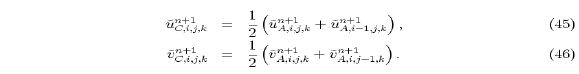
are still required. The trial velocity components on the C grid
 can be calculated from the A-grid velocity
components. Using two-point averaging, for example, we have:
can be calculated from the A-grid velocity
components. Using two-point averaging, for example, we have:
The surface pressure correction  can then be calculated
from the depth integrated horizontal divergence of
can then be calculated
from the depth integrated horizontal divergence of
 over each water
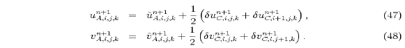
column. The barotropic velocity corrections
over each water
column. The barotropic velocity corrections  can readily be calculated from
through (33) and (34). Interpolations of back to the p-points
yield the total horizontal velocity components on the A grid
can readily be calculated from
through (33) and (34). Interpolations of back to the p-points
yield the total horizontal velocity components on the A grid
 at the end of the time step: