DieCAST and CANDIE both use a finite difference scheme based on
Cartesian coordinates with unevenly-spaced Z-levels in the vertical.
The early version of CANDIE uses the Arakawa C grid for the spatial
discretization with state variables u,v,w and p defined on the
staggered grid illustrated in Figure 1. Note that temperature,
salinity and density are defined at p points and vertical variations
in p are estimated from the overlying density field.
The C grid is widely used in the community [e.g. MICOM of Bleck et al., 1992 and the MIT model of Marshall et al., 1997] because of the ease with which the control volume approach can be implemented, and because the horizontal pressure gradients in the momentum equations and the flux divergences in both the momentum and continuity equations can be calculated to the same numerical accuracy as the other terms in the equations. The main weakness of the C grid, on the other hand, is that the horizontal staggering of the u and v points causes difficulties in estimating the Coriolis terms. DieCAST and CANDIE use different approaches to deal with this difficulty.
In DieCAST, the Coriolis force is treated implicitly  . The
approach suggested by Dietrich et al. [1987, 1990] uses a blend of A
and C grids, thus avoiding the computational burden mentioned above.
The key to this approach is to interpolate the trial velocity
components
. The
approach suggested by Dietrich et al. [1987, 1990] uses a blend of A
and C grids, thus avoiding the computational burden mentioned above.
The key to this approach is to interpolate the trial velocity
components  and
and  to the p points, and update
the advanced trial velocity components at the p points by
integrating equations which include both vertical diffusion and
Coriolis terms (the Ekman spiral equations). The updated velocity is
then interpolated back to the staggered u and v points. Note,
however, that the blend of A and C grids may introduce significant
numerical dissipation, as we now discuss.
to the p points, and update
the advanced trial velocity components at the p points by
integrating equations which include both vertical diffusion and
Coriolis terms (the Ekman spiral equations). The updated velocity is
then interpolated back to the staggered u and v points. Note,
however, that the blend of A and C grids may introduce significant
numerical dissipation, as we now discuss.
Let  , calculated using
(23)-(26)), represent the trial velocity components
at the p-points. They can be calculated, for example, using
two-point averaging of the trial velocity components on the C grid
, calculated using
(23)-(26)), represent the trial velocity components
at the p-points. They can be calculated, for example, using
two-point averaging of the trial velocity components on the C grid
 and
and  by:
by:
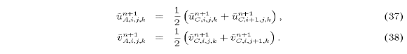
The indices i, j, and k denote the east, north and vertical
coordinates, respectively. The advanced trial velocity components
at the p points  are determined by
the implicit equations (see (27) and (28))
are determined by
the implicit equations (see (27) and (28))
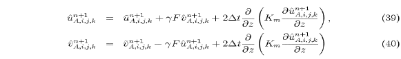
These velocity components are then interpolated back to the u and
v points again to give  and
and  at the u and
v points.
at the u and
v points.
Results show that the smoothing involved in interpolating to the p
points and back again introduces numerical dissipation. For example,
if  and Km=0, differences between
  and
and  are
due solely to the interpolation scheme. It is easily shown that linear
interpolation to the A grid and then back to the C grid is equivalent
to replacing
are
due solely to the interpolation scheme. It is easily shown that linear
interpolation to the A grid and then back to the C grid is equivalent
to replacing  by
by  (i.e. numerical filter weights of (1,2,1)/4). The
smoothing effect is greater for waves with shorter wavelengths. Figure
2 shows the numerical dissipation of wave amplitudes
(i.e. numerical filter weights of (1,2,1)/4). The
smoothing effect is greater for waves with shorter wavelengths. Figure
2 shows the numerical dissipation of wave amplitudes  as a function of the normalized wave number
  , where
 is the grid spacing. The amplitude reduction is about 50\%
for waves with wavelengths of
is the grid spacing. The amplitude reduction is about 50\%
for waves with wavelengths of 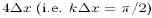 . Further, this dissipation is clearly magnified by reducing
 [Dietrich et al., 1990], since the interpolations are
carried out more times over a given time interval. The
smoothing effect of the interpolation scheme discussed above is
nearly equivalent to harmonic lateral dissipation
[Dietrich et al., 1990], since the interpolations are
carried out more times over a given time interval. The
smoothing effect of the interpolation scheme discussed above is
nearly equivalent to harmonic lateral dissipation  with the non-dimensionalized
diffusion coefficient
with the non-dimensionalized
diffusion coefficient  (see
Figure 2).
(see
Figure 2).
Two approaches have been suggested to reduce this numerical
dissipation. The standard version of DieCAST uses a fourth order
interpolation scheme to reduce the dissipation associated with each
pair of interpolations. Dietrich [1993] shows test cases for a doubly
periodic domain which demonstrate the utility of this approach for
regions which are removed from horizontal boundaries. The effective
filter weights for the fourth order interpolation scheme are
(1,-18,63,164,63,-18,1)/256), corresponding to reduced but still
significant numerical dissipation. Figure 2 shows that the amplitude
reduction using the fourth order interpolation is reduced to about
20\% for waves with wavelengths of  . For
comparison, we also plot the amplitude reduction corresponding
to biharmonic lateral dissipation
. For
comparison, we also plot the amplitude reduction corresponding
to biharmonic lateral dissipation  with the non-dimensionalized diffusion coefficient
  (see Figure 2). Note. however, that
near horizontal boundaries the original version of DieCAST
uses a second order scheme, and the associated dissipation remains
substantial (see the discussion of the canyon test problem in the next
section). Also, this approach still results in dissipation which
increases as
(see Figure 2). Note. however, that
near horizontal boundaries the original version of DieCAST
uses a second order scheme, and the associated dissipation remains
substantial (see the discussion of the canyon test problem in the next
section). Also, this approach still results in dissipation which
increases as  .
.
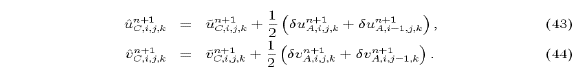
A second modification, which further reduces the dissipation, is to interpolate only the changes in velocity at p points back to the staggered u and v points (e.g., Dietrich et al. [1990]). Let


represent the changes in the trial velocity components at p points
due to the Coriolis and vertical diffusion terms. Interpolating
 back to the u and v points, the advanced
trial velocity components on the C-grid are determined by
back to the u and v points, the advanced
trial velocity components on the C-grid are determined by
If this approach is used, then the dissipation associated with the
interpolations s reduced to zero for the special case  and
and  considered above. Implementation of this
approach in the standard DieCAST model can reduce numerical
dissipation significantly, particularly when small time steps are
required, but some dissipation remains. Further work is required to
improve the accuracy adjacent to boundaries. This issue warrants
further investigation as it may be critical for problems which are
strongly influenced by the boundary conditions [e.g., Haidvogel et
al., 1992; Jiang et al., 1995]. An example from the DieCAST model
which includes both of the above modifications will be discussed in
Section 6.
considered above. Implementation of this
approach in the standard DieCAST model can reduce numerical
dissipation significantly, particularly when small time steps are
required, but some dissipation remains. Further work is required to
improve the accuracy adjacent to boundaries. This issue warrants
further investigation as it may be critical for problems which are
strongly influenced by the boundary conditions [e.g., Haidvogel et
al., 1992; Jiang et al., 1995]. An example from the DieCAST model
which includes both of the above modifications will be discussed in
Section 6.
One further point should be mentioned regarding the treatment of the
Coriolis term in DieCAST. Although  and
and
 are updated using (42) and
(43) with
are updated using (42) and
(43) with  , the surface pressure is computed
using (36) and the associated velocity corrections are
computed using (33) and (34) with
, the surface pressure is computed
using (36) and the associated velocity corrections are
computed using (33) and (34) with  ,
respectively, that is, as if the Coriolis term were being treated
explicitly. As noted by Dietrich et al.[1987], this leads to an error
of order
,
respectively, that is, as if the Coriolis term were being treated
explicitly. As noted by Dietrich et al.[1987], this leads to an error
of order  . Sheng et al. (in preparation) give an
example where this error has significant effect even for F
substantially less than 1.
. Sheng et al. (in preparation) give an
example where this error has significant effect even for F
substantially less than 1.
In CANDIE we choose to treat the Coriolis force explicitly (
), and use the standard four-point averaging of u (v)
[e.g. Heaps, 1972] to determine appropriate estimates at the v (u)
locations for use in (23) and (24). This method is
computationally inefficient if the Coriolis force is treated
implicitly, since it would require  and
and  to be
updated at all grid points simultaneously (see Xu [1994] for an
example where this is done).
to be
updated at all grid points simultaneously (see Xu [1994] for an
example where this is done).